Making Sense of Reshetikhin-Turaev Invariant: $U_q(\mathfrak{sl}_2)$, Kauffman, and Jones

There has been several pieces of common wisdom that I have collected, but have not yet verified. For example, category theories are useful for producing topological invariants. This is a demonstration of this common wisdom, which was substantiated by Sunghyuk Park in his course on quantum topology in Fall 2024. Notes can be found at this link: this short example only uses the more elementary first half of the course. I warn readers that this note is only a execution of the operational procedure without going into deeper conceptual understandings. In fact, most of the content is a direct copy of the lecture notes, so please go and read them for a more thorough exposition. All of the figures are copied from the lecture notes as well. Mathematica code to reproduce all calculations performed in this note can be found here.

Reshetikhin-Turaev: topological invariant of knots

Reshetikhin and Turaev in their seminal paper ^[1] stated the following: given a ribbon category $\mathcal{C}$, one can produce invariants of knots (or more generally ribbon graphs.) A ribbon category needs the following data:

1. Objects and morphisms that make $\mathcal{C}$ a category.

2. (Monoidal.) To make $\mathcal{C}$ monoidal, we need (a) a tensor product structure $\otimes: \mathcal{C}\times\mathcal{C}\to\mathcal{C}$ and (b) an identity object $\mathbb{I}$ s.t. $\mathbb{I}\otimes A = A$ for all $A\in\textrm{Ob}\mathcal{C}$. (Furthermore, some diagrams needs to commute.)

3. (Braided.) To make the monoidal category $\mathcal{C}$ braided, consider the swap map $\tau:$ $\mathcal{C}\times\mathcal{C}\to\mathcal{C}\times\mathcal{C}, (A,B)\to (B,A), (f,g)\to(g,f)$. The opposite tensor product is defined as $\otimes^{\mathrm{op}}=\otimes\circ\tau$. Then, the monoidal category $\mathcal{C}$ is braided if there exists a family of isomorphisms $\beta_{A,B}: A\otimes B\to B\otimes A$, and for all morphisms $f:A\to A', g:B\to B'$, $(g\otimes f)\beta_{A,B}=\beta_{A',B'}(f\otimes g)$. (Furthermore, some diagrams needs to commute.)

4. (Ribbon.) To make the braided category $\mathcal{C}$ a ribbon category, one needs two concepts: one is the concept of duality and rigidity, and the other is the concept of twist. A monoidal category is right/left rigid if all objects $A$, there are right/left duals $A^*$ / $^*\! \!A$. For left rigid categories, we have the right cup and cap morphisms: $\vec{\cup}_A:\mathbb{I}\to$ $^* \! \!A\otimes A$ and $\vec{\cap}_A: A\otimes \ ^* \! \!A\to \mathbb{I}$. They need to satisfy zigzag identities. There also needs to be a compatible twist $\theta$, i.e. a natural family of isomorphisms $\theta_A:A\to A$, for which $\theta_{A\otimes B}=\beta_{B,A}\beta_{A,B}(\theta_A\otimes\theta_B)$.

If all four items of the data are provided, the category $\mathcal{C}$ is a ribbon category.

Now, Reshtikhin-Turaev claims the following. Given a ribbon graph, one can label its ribbons using objects of $\mathcal{C}$ (i.e. a coloring). Then, we may have the following dictionary (copied from the lecture notes):

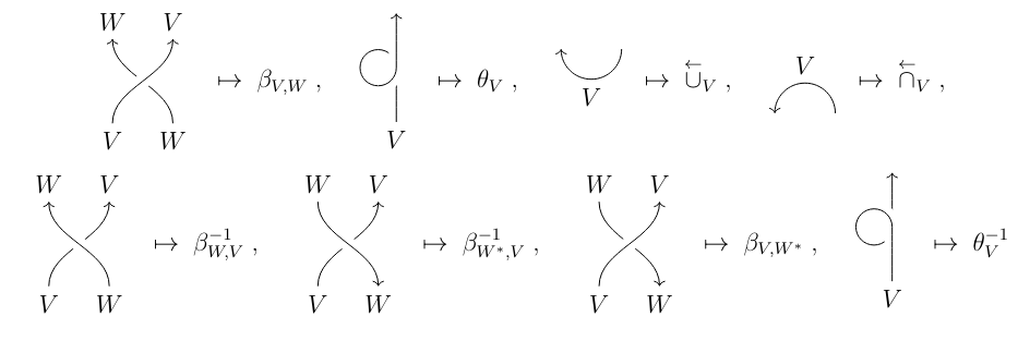
With this dictionary, one can assign basically a number to a knot – which is invariant under general knot invariant moves.

Ribbon Category from Hopf algebra data

These ribbon categories are still a bit abstract for me. What's great is that you can construct them from something a little bit more concrete called the Hopf algebra. The Hopf algebra first needs to be a bialgebra: i.e. both an algebra and a coalgebra. A bialgebra is a tuple $(B,\mu,\eta,\Delta,\epsilon)$, where $\mu$ the product and $\epsilon$ the unit make $B$ an algebra, and $\Delta$ the coproduct and $\eta$ the counit make $B$ a coalgebra, and furthermore $\Delta$ and $\epsilon$ are algebra morphisms. By coproduct, we mean a linear map $B\to B\otimes B$. It has to satisfy the dual of the associativity rule: $(\Delta\otimes \textrm{id})\Delta = (\textrm{id}\otimes\Delta)\Delta$. The counit $\epsilon: B\to\mathbb{k}$ is such that $(\epsilon\otimes \textrm{id})\Delta=\textrm{id}=(\textrm{id}\otimes \epsilon)\Delta$.

A Hopf algebra is a bialgebra $B$ such that the identity map is invertible in the convolution algebra $\textrm{End}(B)$. In plain words, there exists an antipode $S\in\textrm{End}(B)$ s.t.

Some quick examples to keep in mind: the group algebra $\mathbb{k}[G]$ is a cocommutative Hopf algebra where

The dual algebra is also a Hopf algebra if $G$ is finite:

For Hopf algebra $B$, the category $B-\textrm{Mod}^{\textrm{fin}}$ is naturally a rigid monoidal category. The coproduct $\Delta$ provides the action of $H$ on tensor products, and $S$ provides the action on the dual modules.

To make a Hopf algebra $B$ braided, one equips it with an invertible element $R\in B\otimes B$ known as the univeral $R$-matrix. It needs to satisfy a bunch of properties. Most importantly, it makes $B-\textrm{Mod}$ naturally a braided monoidal category, with the braid morphisms given by:

where $\sigma$ exchanges the objects.

Finally, let's suppose $S$ the antipode is invertible. Then, we can consider the element

One can prove that $uS(u)$ is central. Its square root $\nu$ is called the ribbon element:

and using it we can define the twist morphisms:

Concrete example: $U_q(\mathfrak{sl}_2)$

$U_q(\mathfrak{sl}_2)$ is a quantum group. I do not know why it is called this way. Semantically, it seems that it can be interpreted as a "quantized" version of the Lie algebra $\mathfrak{sl}_2$, which we will explain below.

$U_q(\mathfrak{sl}_2)$ is a $\mathbb{C}(q)$-algebra generated by $E\sim \sigma^+$, $F\sim\sigma^-$, and $K^{\pm 1}\sim q^{\pm \sigma_z}$. It is also useful to denote $H\sim \sigma_z$. They have the following relations:

It has a Hopf algebra structure:

The universal $R$-matrix can be written as

Although this is formally an infinite sum, once we restrict to a finite dimensional representation $V$, the sum can be truncated to $n\sim \textrm{dim}(V)$. $[n]!$ is the quantum version of factorial, $[n]! = \prod_{m\leq n}[m]$, where $[m]$ is quantum $m$:

One can determine the ribbon element $\nu$ next by determining $u$, and computing $uS(u)$. We indeed do this in the mathematica notebook. On the other hand, it is interesting to use the following simpler formula:

Kauffman bracket and Jones polynomial generated from RT invariants of $U_q(\mathfrak{sl}_2)$

Basic knot invariant technology

The Kauffman bracket $\left\langle L \right\rangle$ is defined with these relations:

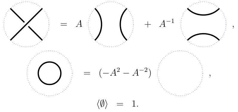
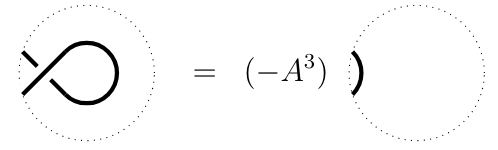
where the first relation is called the skein relation. The Kauffman bracket is not invariant under all the knot equivalence move; particularly, if I twist a strand of the knot (R1 of the Reidemeister move), the Kauffman bracket transforms as

The Jones polynomial is created to cure this:

where $w(L)$ is the writhe of the link that counts the number of signed crossings. Jones polynomial is an invariant of knots, whereas the Kauffman bracket is an invariant of framed links.

The Jones polynomial is generated by these relations:

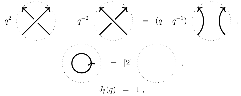
The first one is also called the skein relation.

Calculating RT invariants

Now we will color knots by the 2-dimensional representation of $U_q(\mathfrak{sl}_2)$, spanned by $\ket{\uparrow}$ and $\ket{\downarrow}$.

The universal $R$-matrix significantly simplifies. Particularly, we can show that

Furthermore, $\nu = q^{-3/2}$.

Now, we try to prove the skein relation for Kauffman brackets. We first color the diagrams: we color the two ends at the bottom with $V_2$ (i.e. arrows going in), and the two ends at the top also $V_2$ (i.e. arrows going out). This means that for the diagram on the left we have $\beta_{V_2,V_2}=\sigma_{V_2,V_2} R$; on the right, the first diagram is the identity, but the second diagram is confusing. What should we do when two ingoing arrows meet?

Note that we only know what happens when one arrow goes in and one goes out; those are the cup and cap morphisms. This means that we need to flip the arrows for one of the top ends and one of the bottom ends. This can be done using the following $U_q(\mathfrak{sl}_2)-\textrm{Mod}$ isomorphism $g:V_2\to V_2^*$:

Thus, for example, the bottom portion where both arrows are going in can be computed as $\vec{\cap}_{V_2}\circ(\textrm{id}\otimes g)$. From this, we can successfully verify the skein relation (up to a minus sign):

To compute the Jones polynomial of the unknot, one splits it into a left cap and a right cup. The composition of these morphisms will give $q+q^{-1}=[2]$, which also agrees up to a minus sign. This thus proves that the RT invariant of links colored by $V_2$ reproduces the Kauffman bracket.

The procedure to produce the Jones polynomials is a bit trickier. For the first diagram on the left of the skein relation one needs to use $q^{-3/2}\beta_{V_2,V_2}=(\theta_{V_2}^{-1}\otimes \textrm{id})\beta_{V_2,V_2}$, and for the second diagram one needs to use $q^{3/2}\beta_{V_2,V_2}^{-1}=(\theta_{V_2}\otimes \textrm{id})\beta_{V_2,V_2}^{-1}$. The reason for this is exactly the "covariance" under the R1 move, but I do not know how to mathematically justify this from the RT perspective. After all, the RT invariant is an invariant of ribbon diagrams, which cares about the twisting of ribbons, rather than knots.

More examples, such as a calculation of the Jones polynomial of the Hopf link, where $J_L(q)=q^{-6}+q^{-4}+q^{-2}+1 = (q+q^{-1})(q^{-1}+q^{-5})$, can also be found in the notebook.