Gel'fand-Yaglom Trick: The Only Trick You Need for Functional Determinants?

This note originates from discussions with Daniele Guerci and Eslam Khalaf on Wronskians, during which Eslam mentioned this trick that is simply too powerful and magical to miss. This note mainly follows the structure of ^[1], and the original references are ^[2][3].

Functional Determinants

These are objects that appear in your path integrals. For example, the simplest path integrals are the path integrals that appear in $0+1$ dimensional quantum mechanics:

$$\mathcal{Z}=\int \mathcal{D}x e^{-S[x]}$$

where one imposes the conditions that $x(0)=x(\beta)$. If the action is quadratic in $x$, then we may diagonalize the kernel of the Gaussian and perform the Gaussian integration. Particularly, if

$$S[x]=\int_0^\beta d\tau \ x(\tau) (\partial_{\tau}^2+V(\tau))x(\tau),$$

then we can write down the partition function as

$$\mathcal{Z} = \det(\partial_{\tau}^2+V(\tau))^{-1/2}.$$

The same thing happens in quantum field theories. If we have a complex bosonic field $\phi$, then its coherent state path integral gives

$$\mathcal{Z} = \int \mathcal{D}\phi e^{-\int d\tau \bar{\phi}(\partial_\tau+\mathcal{H})\phi} = \det(\partial_\tau+\mathcal{H})^{-1},$$

whereas the fermionic path integral of a fermionic field $\psi$ gives

$$\mathcal{Z} = \int \mathcal{D}\psi e^{-\int d\tau \bar{\psi}(\partial_\tau+\mathcal{H})\psi} = \det(\partial_\tau+\mathcal{H}).$$

We have to recall that the boundary conditions are important for the path integrals: for the bosonic case, one should use the periodic boundary conditions $\phi(0)=\phi(\beta)$, whereas for the fermionic case one should use anti-periodic boundary conditions $\psi(0)=-\psi(\beta)$. Using periodic boundary conditions for fermions corresponding to inserting $(-1)^F$ in the path integral, and thus we would be computing the Witten index.

Now let's recall how determinants are defined. Consider an ordinary matrix – or linear operator $\mathcal{M}$. Let's say it is fully diagonalizable (after all they are dense – apply a perturbation and break all the degeneracies so you don't get Jordan blocks), by which we mean

$$\mathcal{M}\phi_n = \lambda_n \phi_n,$$

and furthermore let us assume that the spectrum is bounded from below, $0<\lambda_1<\lambda_2<\dots$ The determinant can be written as the product of all the eigenvalues:

$$\det \mathcal{M} = \prod_n \lambda_n.$$

One should immediately be aware that this is not a good thing to do for general linear operators – after all, the infinite product that we would be computing should be infinitely large. But that is usually not a problem for mathematicians or physicists.

Let us now define an auxiliary wavefunction called the $\zeta$ function, corresponding to the operator $\mathcal{M}$. Following the convention in ^[1], I will suppress the $\mathcal{M}$ dependence on $\zeta$, but it's good to keep in mind.

The $\zeta$ function is defined as

$$\zeta(s)\equiv \mathrm{Tr}(\mathcal{M}^{-s})=\sum_{n}\frac{1}{\lambda_n^s}.$$

When the eigenvalues are positive integers, you get the usual Riemann $\zeta$ function. For the Landau level, you get the Hurwitz $\zeta$ function with shift $1/2$ – $\lambda_n=n+1/2$. It would be interesting to see if there are natural ways to build quantum mechanical Hamiltonians for general Dirichlet $L$ functions, but that's for another day probably.

One can compute the derivative of the $\zeta$ function at $s=0$:

$$\zeta'(0)=-\sum_n\log \lambda_n.$$

Thus, the functional determinant of $\mathcal{M}$ can be related to the derivative:

$$\det \mathcal{M} = \exp(-\zeta'(0)).$$

It would have been fantastic if the $\zeta$ function is well defined at $s=0$. In fact, one can see that for the operator $\mathcal{M}=-\nabla^2$ in $d$ dimensions,

$$\zeta(s) \sim \int_{|k|>1} \frac{d^d k}{k^{2s}},$$

which is not convergent when $s\left.<\right. d/2$ in general!

To compute the $\zeta$ function (and the determinant), we need to introduce proper regularizations. Particularly we introduce the trace of the heat kernel:

$$K(t)=\mathrm{Tr} e^{-\mathcal{M}t}=\sum_{n}e^{-\lambda_n t}$$

which should be generally (more) convergent given that the spectrum $\{\lambda_n\}$ is bounded below. Then, one may perform the Mellin transform to get the zeta function:

$$\zeta(s) = \frac{1}{\Gamma(s)}\int_0^\infty dt \ \ t^{s-1} K(t).$$

(We note that the original Riemann $\zeta$ function is analytically continued onto the complex plane using exactly this formula, with $K(t) = \sum e^{-nt}=(e^{t}-1)^{-1}$, and the Epstein $\zeta$ functions with $K(t)$ being some sort of Jacobi $\theta$ functions. Indeed, if one considers the Mellin transform of the $\theta$ function, one may relate $\zeta(s)$ to $\zeta(1-s)$ – but that's also for another day.)

We have now handwavingly defined the functional determinant of a general linear operator $\mathcal{M}$. On to the calculations!

The Gel'fand-Yaglom Trick

A Magical function $\mathcal{F}$

Let's say that you have some sort of magical oracle, who provides you the following function $\mathcal{F}$. $\mathcal{F}(\lambda)$ exactly has the eigenvalues of $\mathcal{M}$ as its simple zeros: $\mathcal{F}(\lambda)=0$ if and only if $\lambda$ is in the spectrum of $\mathcal{M}$, and $\mathcal{F}'(\lambda_n)\neq 0$. One may say that they can easily come up with such a function: just take $\mathcal{F}(\lambda) = \det(\mathcal{M}-\lambda)$. Indeed, that is probably right, but this has simply translated the calculation of one functional determinant into another one – which is strictly harder, because $\mathcal{F}(0) = \det(\mathcal{M})$ in this case! Indeed, we will soon prove that $\det \mathcal{M}\propto \mathcal{F}(0)$, and we will provide another shortcut to calculate $\mathcal{F}(0)$.

but first let's see what you can do with a general function $\mathcal{F}$ with this property. Let us consider its logarithmic derivative:

$$\frac{d\log \mathcal{F}(\lambda)}{d\lambda} = \frac{\mathcal{F}'(\lambda)}{\mathcal{F}(\lambda)}.$$

The logarithmic derivative of $\mathcal{F}$ has simple poles at $\lambda_n$ with residue $1$, irrespective of what $\mathcal{F}$ is. This can be seen as the trace of the resolvent of $\mathcal{M}$:

$$\frac{d\log \mathcal{F}(\lambda)}{d\lambda} =\mathrm{Tr} R(\lambda;\mathcal{M})=\mathrm{Tr} \frac{1}{\lambda - \mathcal{M}}.$$

Thus, the zeta function can be written as an integral with the following contour:

$$\zeta(s) =\frac{1}{2\pi i}\int d\lambda \frac{1}{\lambda^s} \mathrm{Tr} \frac{1}{\lambda - \mathcal{M}} = \frac{1}{2\pi i}\int d\lambda \frac{1}{\lambda^s}\frac{d\log \mathcal{F}(\lambda)}{d\lambda}$$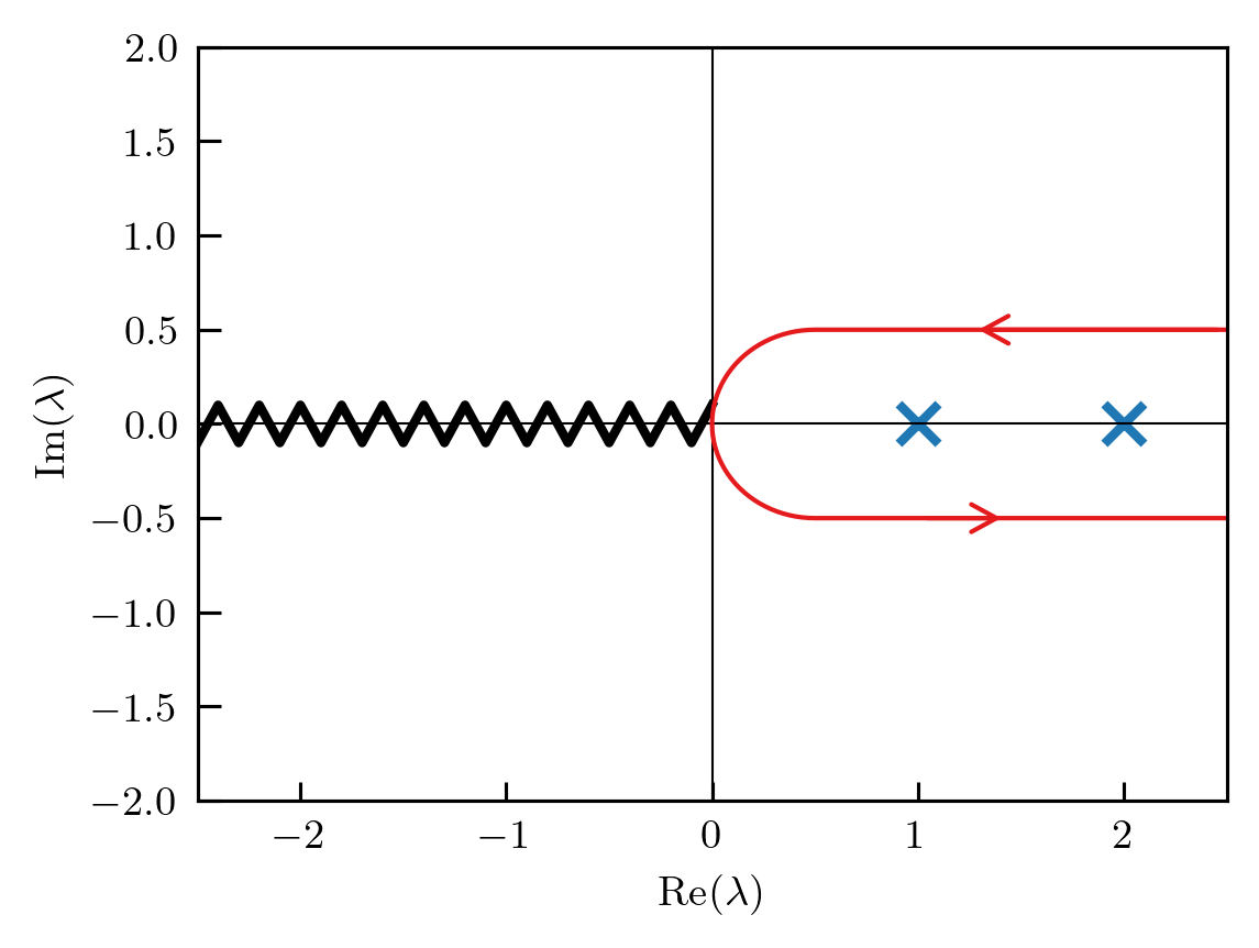

where the blue crosses represent the poles of the resolvent and the black wavy line represent the branch cut of the function $1/\lambda^s$. As one expects, we now deform the contour of the integral:

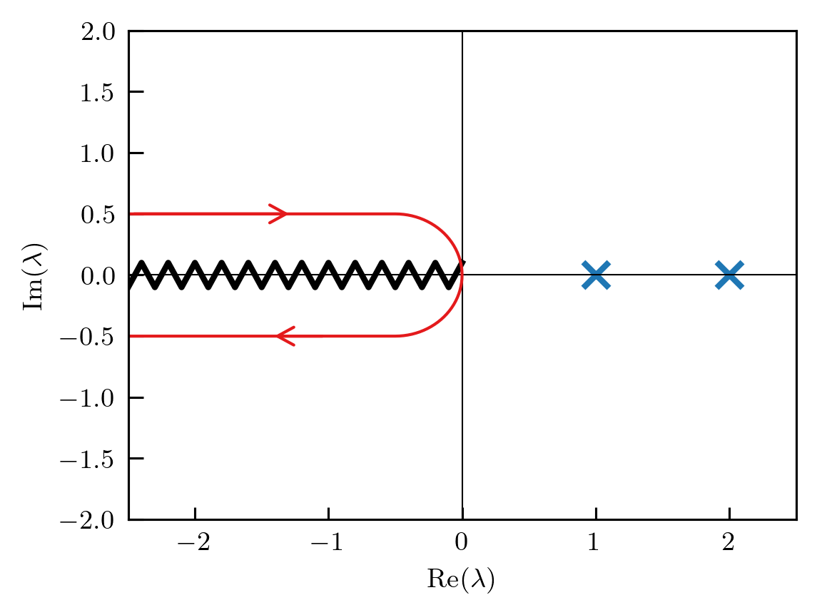
Thus the integral becomes

$$\zeta(s) =\int_0^{-\infty} d\lambda \left(\frac{1}{(\lambda-i\epsilon)^s}-\frac{1}{(\lambda+i\epsilon)^s}\right)\frac{d\log \mathcal{F}(\lambda)}{d\lambda} = \frac{\sin \pi s}{\pi}\int_0^{-\infty} d\lambda \frac{1}{|\lambda|^s}\frac{d\log \mathcal{F}(\lambda)}{d\lambda}$$

Thus we may simplify the definition of $\zeta'(0)$:

$$\zeta'(0) = -\log\mathcal{F}(0)+\log\mathcal{F}(-\infty)$$

The functional determinant can thus be expressed as

$$\det\mathcal{M} = \frac{\mathcal{F}(0)}{\mathcal{F}(-\infty)}.$$

Indeed, in practice what one would usually compute is a ratio of functional determinants, which usually converges to something finite:

$$\frac{\det\mathcal{M}}{\det\mathcal{M}_{\textrm{free}}} = \frac{\mathcal{F}(0)}{\mathcal{F}_{\textrm{free}}(0)}.$$

We have cancelled out the infinite contributions. In fact, one can probably think of this precisely as the regulator for calculating this functional determinants.

$\dots$ but where can I buy the magical function?

So in the last section we have seen that you want a magical $\mathcal{F}(\lambda)$ with simple zeros precisely at the spectrum of the operator $\mathcal{M}$. Let us now construct one.

In this section, we will consider the limited case for Dirichlet boundary conditions: $\phi(0)=\phi(\beta)=0$, and quadratic derivative operators:

$$\mathcal{M}=-\partial_\tau^2+V(\tau).$$

Let's consider the solution of the following differential equation:

$$\mathcal{M}u_{\lambda}(\tau) = \lambda u_{\lambda}(\tau),$$

where $u_{\lambda}(0)=0, u'_{\lambda}(0)=1$. In general, since this is just an ordinary second order differential equation with correctly specified boundary conditions. The boundary conditions on $u'(0)$ is simply a normalization – it will not be important. Here comes the magic.

Consider the quantity $u_\lambda(\beta)$. I claim that this function is zero precisely for $\lambda$ that lives in the spectrum of $\mathcal{M}$ with the boundary conditions $\phi(0)=\phi(\beta)=0$!

One side is easy to see: if $u_{\lambda}(\beta)=0$, then it becomes an eigenstate with the correct boundary condition, and thus $\lambda$ is in the spectrum.

For the other side, consider the Wronskian $W(\phi_n,u_{\lambda}) = \phi_n'u_{\lambda}-u_{\lambda}'\phi_n$. Now, $W'(\tau) = \phi_n''u_{\lambda}-u_{\lambda}''\phi_n=(\lambda-\lambda_n)\phi_n u_\lambda$. Now we integrate and find out:

$$u_{\lambda}(\beta) = \frac{W(\beta)-W(0)}{\phi_n'(\beta)} = \frac{\lambda-\lambda_n}{\phi_n'(\beta)}\int_0^\beta d\tau \phi_n u_\lambda$$

and thus, if $\lambda=\lambda_n$, $u_{\lambda}(\beta)=0$.

We have thus proven that $u_{\lambda}(\beta)$ is our magic function:

$$\mathcal{F}(\lambda)=u_{\lambda}(\beta)!$$

From the discussion above, we know that $\mathcal{F}(\lambda)$ is almost $\det(\mathcal{M}-\lambda)$. This equivalence can be most easily understood as a Liouville argument: $u_{\lambda}(\beta)$ has the same zeros as $\mathcal{F}(\lambda)$ and $\det(\mathcal{M}-\lambda)$, and all of them are analytic in $\lambda$, which means that they must be the same up to a (possibly infinite) constant – which gets cancelled when one calculates the ratio of determinants.

More boundary conditions

We have now obtained the functional determinant for Dirichlet boundary conditions. But the boundary conditions that we really care about are periodic or antiperiodic boundary conditions. Fortunately one can still perform the same procedure. Let us write down the general form of boundary conditions as

$$M \left(\begin{array}{c}\phi(0)\\ \phi'(0)\end{array}\right) + N \left(\begin{array}{c}\phi(\beta)\\ \phi'(\beta)\end{array}\right)=0$$

For Dirichlet,

$$M = \left(\begin{array}{cc}1 & 0\\ 0 & 0\end{array}\right), N=\left(\begin{array}{cc}0 & 0\\ 1 & 0\end{array}\right).$$

For Neumann,

$$M = \left(\begin{array}{cc}0& 0\\ 0 & 1\end{array}\right), N=\left(\begin{array}{cc}0& 1\\ 0 & 0\end{array}\right).$$

For periodic,

$$M = \left(\begin{array}{cc}1& 0\\ 0 & 1\end{array}\right), N=-\left(\begin{array}{cc}1& 0\\ 0 & 1\end{array}\right).$$

For antiperiodic,

$$M = \left(\begin{array}{cc}1& 0\\ 0 & 1\end{array}\right), N=\left(\begin{array}{cc}1& 0\\ 0 & 1\end{array}\right).$$

One can then construct two solutions: $u_{\lambda 1}(0)=1,u'_{\lambda 1}(0)=0$, and $u_{\lambda 2}(0)=0,u'_{\lambda 2}(0)=1$. If any linear combinations of the two solutions satisfy the boundary conditions, then $\lambda$ is in the spectrum. We simply need to express the condition that there exist a linear combination as an algebraic equation.

Indeed, one can check that

$$\mathcal{F}(\lambda)=\det\left(M+N\left(\begin{array}{cc}u_{1\lambda}(\beta)& u_{2\lambda}(\beta)\\ u_{1\lambda}'(\beta) & u_{2\lambda}'(\beta)\end{array}\right)\right)$$

correctly hits zero as the boundary condition is met (and thus we have $\lambda=\lambda_n$ for some $n$). The functional determinant is therefore

$$\det\left(-\partial_\tau^2+V(\tau)\right)=\mathcal{F}(0)=\det\left(M+N\left(\begin{array}{cc}u_{1,\lambda=0}(\beta)& u_{2,\lambda=0}(\beta)\\ u_{1,\lambda=0}'(\beta) & u_{2,\lambda=0}'(\beta)\end{array}\right)\right).$$

Examples: bosons and fermions

In this section we will compute functional determinants for a free boson and a free fermion, both at frequency $\omega$. The boson partition function is

$$\mathcal{Z}_b =\frac{\det(\partial_\tau+\omega)^{-1}_{P}}{\det(\partial_\tau)^{-1}_{P}},$$

whereas the fermionic partition function is

$$\mathcal{Z}_f = \frac{\det(\partial_\tau+\omega)_{AP}}{\det(\partial_\tau)_{AP}} .$$

One might think that these are single derivative operators and it would not be possible to calculate the partition functions. This is not true. In fact one needs to apply a time reversal to the determinant, which leaves the boundary conditions invariant. This flips the sign of $\partial_\tau$. Multiplying them together and taking the square root, we get

$$\mathcal{Z}_b = \frac{\det(-\partial_\tau^2+\omega^2)^{-1/2}_{P}}{\det(-\partial_\tau^2)^{-1/2}_{P}} , \quad \mathcal{Z}_f =\frac{\det(-\partial_\tau^2+\omega^2)^{1/2}_{AP}}{\det(-\partial_\tau^2)^{1/2}_{AP}} .$$

Let us use the tricks learned in the last section to calculate the determinants. The two solutions we have are

$$u_{1,\lambda=0}(\tau)=\cosh\omega\tau, \quad u_{2,\lambda=0}(\tau) = \frac{\sinh\omega\tau}{\omega}.$$

Plugging them into the formulas above, we get

$$\det(-\partial_\tau^2+\omega^2)_P = -\sinh^2\frac{\beta\omega}{2},\quad \det(-\partial_\tau^2+\omega^2)_{AP}=\cosh^2\frac{\beta\omega}{2}.$$

One might be confused why I am getting something that is negative when I'm computing a positive product: the honest answer is I don't know. But very nicely, the negative sign drops out when we consider the ratio of determinants. (Also we don't consider anomalies here so I can ignore phases of the partition function.)

$$\mathcal{Z}_b =\frac{\beta\omega}{2\sinh \frac{\beta\omega}{2}},\quad \mathcal{Z}_f = \cosh\frac{\beta\omega}{2}.$$

which is exactly what you expect. More examples can be found in ^[1], but that's beyond the scope of this post.

References

[1]	G. Dunne, Functional Determinants in Quantum Field Theory (2009). link

[2]	I. M. Gel'fand and A. M. Yaglom, Integration in Functional Spaces and its Applications in Quantum Physics (1960). DOI

[3]	S. Levit and U. Smilansky, A theorem on infinite products of eigenvalues of Sturm-Liouville type operators (1977). DOI